Adding cost uncertainty to the project schedule

Understanding and managing the total cost of a project is critical to its success. The timing of those costs can also be very important – large up-front costs followed by long delays may put enormous strains on a company’s cashflow, even if the project does not exceed its budget. Tamara offers a comprehensive suite of tools to incorporate the uncertainty and risk associated with costs and their timing, and provides a range of reports to help understand the cashflow risk over time as well as the risk on the total cost to completion.

The simulation results on cost and completion dates from Tamara can be further used in financial models built with ModelRisk, if required, so that a business can build a complete understanding of the financial viability of a project.

The following description provides a list of the different ways that Tamara can incorporate cost-related risk. Follow the links to review more details on each method.

Risk events

A risk event is an event that may or may not occur - like a fire, an earthquake, a power outage or a strike. Tamara recognizes three different types of risk event:

1. Task-specific risk events – these cause a delay to a specific task(s) and/or an additional cost that occurs during the execution of that task(s)
2. Unplanned work– extra work that becomes necessary but was not in the original plan
3. Disruptions – delays to the whole project, or a section of the project, during its execution

For each type of risk event one may include a cost impact. Tamara will automatically incorporate any additional time-based costs that result from extensions to a task's duration.

Task duration uncertainty

If a task requires resources for which the cost is dependent on how long those resources are used, then any uncertainty in the duration of that task translates into an uncertainty about the resource-related costs. Tamara will automatically account for this time-related resource cost uncertainty when a resource has been allocated to a task.

Adding uncertainty to resource-related costs

The uncertainty in resource-related costs is driven by the uncertainty in the amount of time a resource is allocated to a specific task, accounted for in the various task duration modeling tools in Tamara, and by the uncertainty in the cost of each resource required to complete the specific task.

Tamara determines an average daily rate for the aggregated costs of all resources attached to a specific task, and then applies that daily rate to the simulated uncertain task duration.

For example, if a task has a 12 days duration in the original schedule, to which had been allocated 30 person days of electrical technicians and 10 days or telecommunications engineers at $400 and $600 per day respectively, Tamara would proceed as follows:

Daily rate for electrician cost = (30 x $400) / 12 days = $1,000 / day.

Daily rate for telecoms engineer cost = (10 x $600) / 12 days = $500 / day.

Then Tamara applies the simulated duration of the task, and any uncertainty in the daily rate to give the total cost for the task. For example, if Tamara simulates that the actual electrician rate could be 5% less, the telecoms 10% more, and the task could take 30% longer, it would calculate the total cost as:

                Total cost = ( $1,000/day * (100%-5%) + $500/day * (100%+10%) ) * (12 days * (100%+30%)) = $23,400

 

We begin by specifying definitions in the Cost Uncertainty Definitions window:

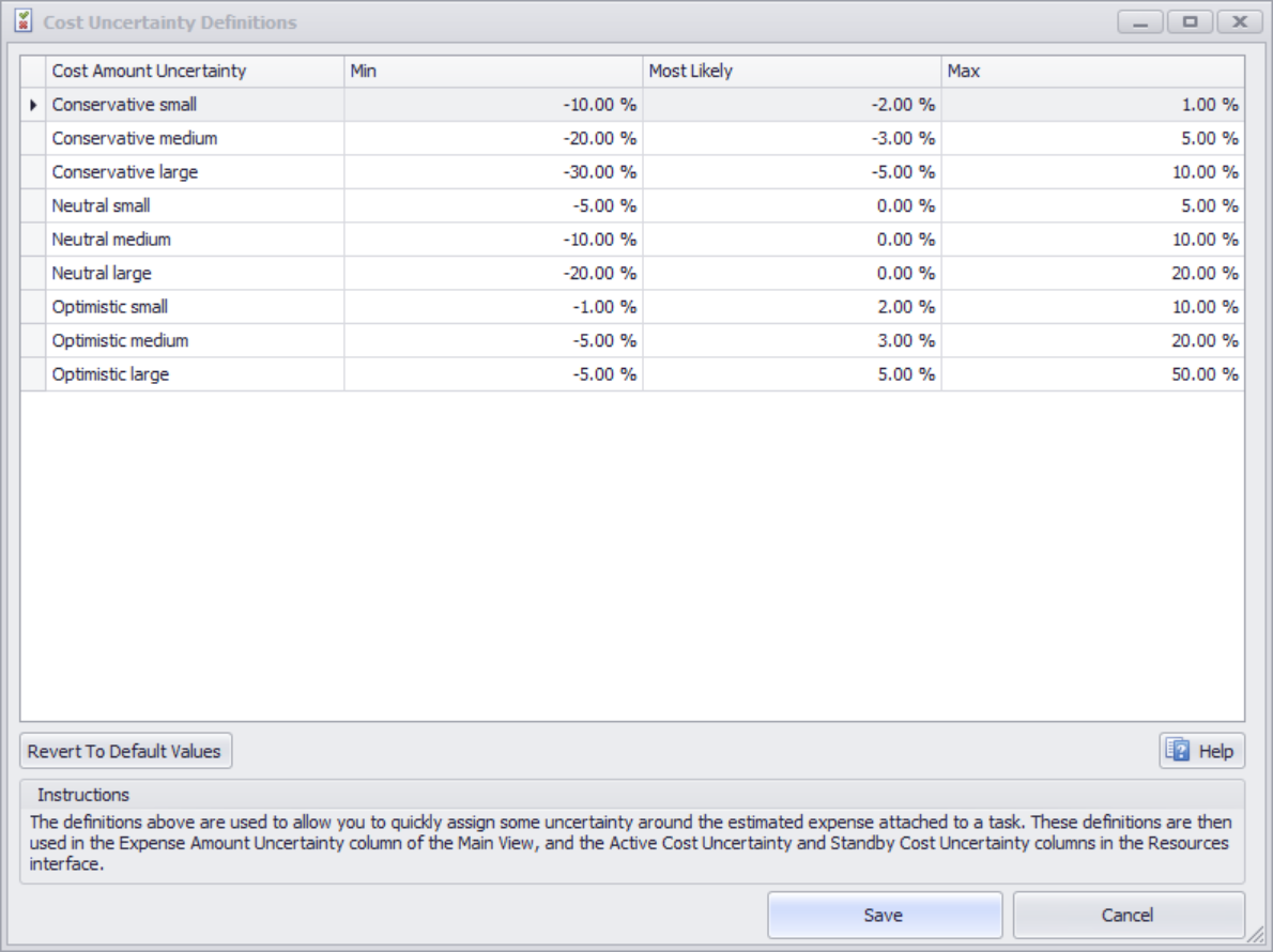
Analogous to the work amount uncertainty definitions, this allows one to define some descriptive terms to apply to costs. These terms are then applied to resource costs and to expenses.

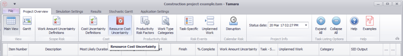
Tamara automatically uses any resource cost and allocation data available in the imported schedule model. Tamara gathers together all the resources present in the imported schedule and presents them in the Resource Cost Uncertainty table, accessed by clicking the Resource Cost Uncertainty icon in the Main view tab:

The Resource Cost Uncertainty table organizes the resources into materials and labor according to the imported schedule designation:

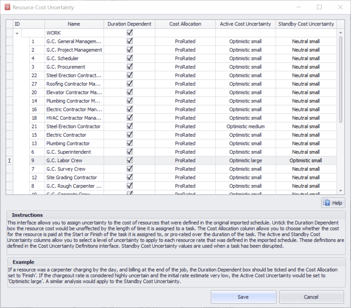
The first column specifies whether the cost is related to the duration of a task. By default, this is checked on – unchecking it will make Tamara calculate the cost from the original unrisked schedule and apply any uncertainties to it.

The second column specifies at what point the cost is paid. By default, the cost of all resources are given a ‘ProRated’ allocation, meaning that they are assumed to occur evenly in time over the duration of a task, as shown above in the Cost Allocation field. The user can choose between three Cost Allocation options – Start, Finish and ProRated:

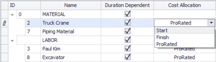
Start – the cost occurs when the task is started

Finish – the cost occurs when the task is completed

ProRated – the cost occurs evenly between the start and finish of the task

For example:

• Transporting onsite and erecting a crane (material) might incur a cost that is paid at the start of the first task that requires the crane = Start

• Dismantling and transporting offsite a crane (material) might incur a cost that is paid at the finish of the last task that requires the crane = Finish

• Truck operator (labor) costs might be paid evenly during tasks in which the crane is being used  = Pro-rated

• Windows (material) might be delivered on to a construction site in one batch and be paid for on delivery, even though the installation of the windows is performed in several stages over different tasks = Start

• Installation by a contractor of the IT system at a construction site might involve payment for the equipment (material) at the start of the installation (= Start), but the installation costs (labor) might be paid for when the installation is complete (= Finish).

The third column, Active Cost Uncertainty, specifies the degree to which the resource cost used in the original model is uncertain. It applies this cost to the resource when that resource is attached to a task that is being worked on.

The last column, Standby Cost Uncertainty, specifies the degree to which the resource cost used in the original model is uncertain when that resource is idle (i.e. during a disruption event).

 

Adding uncertainty to expense-related costs

Tasks can have additional expenses attached to them within the imported schedule. These expenses can be set in Primavera or MS Project to occur at the beginning, end or evenly throughout the execution of the task.

Tamara replicates this logic and timing of the expense, adjusting remaining expenses according to the level of completion of the task, by multiplying the expense value by the following values:

Level of completion	Initial expense	Continuous expense	Final expense
Not started	1	1	1
Fraction of work (p) completed	0	(1-p)	1
Coompleted	0	0	0

 

In other words:

• Expenses for completed tasks are ignored

• Expenses for tasks not yet started are included at full value

• If a faction p of the task is complete, an expense occurring at the beginning of a task is ignored, an expense occurring at the end of the task is included at full value, and for an expense occurring evenly over the task’s duration, a fraction (1-p) of that expense is included.

For these revised expense values, the user can apply an Expense Amount Uncertainty factor to the total of the expenses, using the procedure described below.

In the Main View window of Tamara, if there are any expenses allocated to a particular task the total expenses (incurred at the start of the task, pro-rated across the task duration and/or incurred at the task finish) are shown in the Expenses column. In the column to its right (Expense Amount Uncertainty) one may select one of the Cost Uncertainty Definitions from a drop-down list:

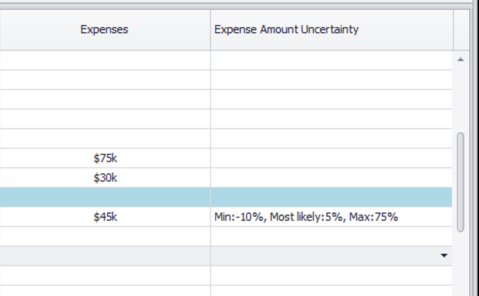
Selecting one of these phrases will apply the appropriate uncertainty to the total expenses. For some expenses, none of the definitions may reflect the uncertainty. This usually occurs when there is an expense for which the uncertainty distribution has a particularly long right tail. In such situations, select Custom from the bottom of the list.  This will open the following dialog box:

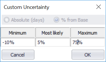
You can now enter a distribution specific to that expense as a percentage variation around the base estimate. The cell will then show these three value for easy reference:

You can edit the entered values by selecting the cell again, removing the uncertainty by clicking the blank line, then reentering a new Custom range.

You can quickly assign expense uncertainty to a set of tasks, which is very useful if you have a large schedule. In the default view, where tasks are shown at various levels (parent and child), selecting a parent task and then picking an uncertainty description will assign this expense uncertainty to all child tasks below it. For large schedules, you may find that the easiest approach is to first define the expense amount uncertainty at Level 1 or 2, and then edit for individual sub-tasks where there are exceptions.